One Position, Four Bets: Turning Conviction Into Tradeable Risk
A position-level view of sizing, hedging, and conviction, built on one additive cascade.
By Conrad Gann — Founder, RiskModels.app
Trailing 12 months: April 21, 2025 – April 21, 2026. All analysis as of 2026-04-21.
Concentrated PMs — and the allocators and risk teams evaluating them — think name-by-name, not factor-by-factor. The question isn't "how is the book tilting"; it's "what is this position actually built to deliver, and what discrete bets inside it can I size and hedge separately?" Portfolio-down risk tools aggregate first, then decompose. They answer the aggregate question well, but not the position-level one. Without this view, two positions with the same label can carry fundamentally different exposures — a PM can express the right thesis with the wrong instrument, and only see it after the fact.
Position-up decomposition runs the math the other way. Each ticker is broken into four additive, orthogonal layers:
- L1 — market (SPY)
- L2 — sector, stripped of L1 (e.g. XLK net of SPY)
- L3 — subsector, stripped of L1 and L2 (e.g. SMH net of SPY and XLK, as a tradable proxy)
- L3 residual — what no ETF replicates
Because each layer is stripped of the layers above it, the same cascade drives both Return Attribution (percentage points of realized return, summing exactly to gross) and Risk Attribution (explained risk by layer — variance fractions from orthogonal regressions, summing to ~100%). One object, two views: realized return and layer-wise explained risk for hedging.
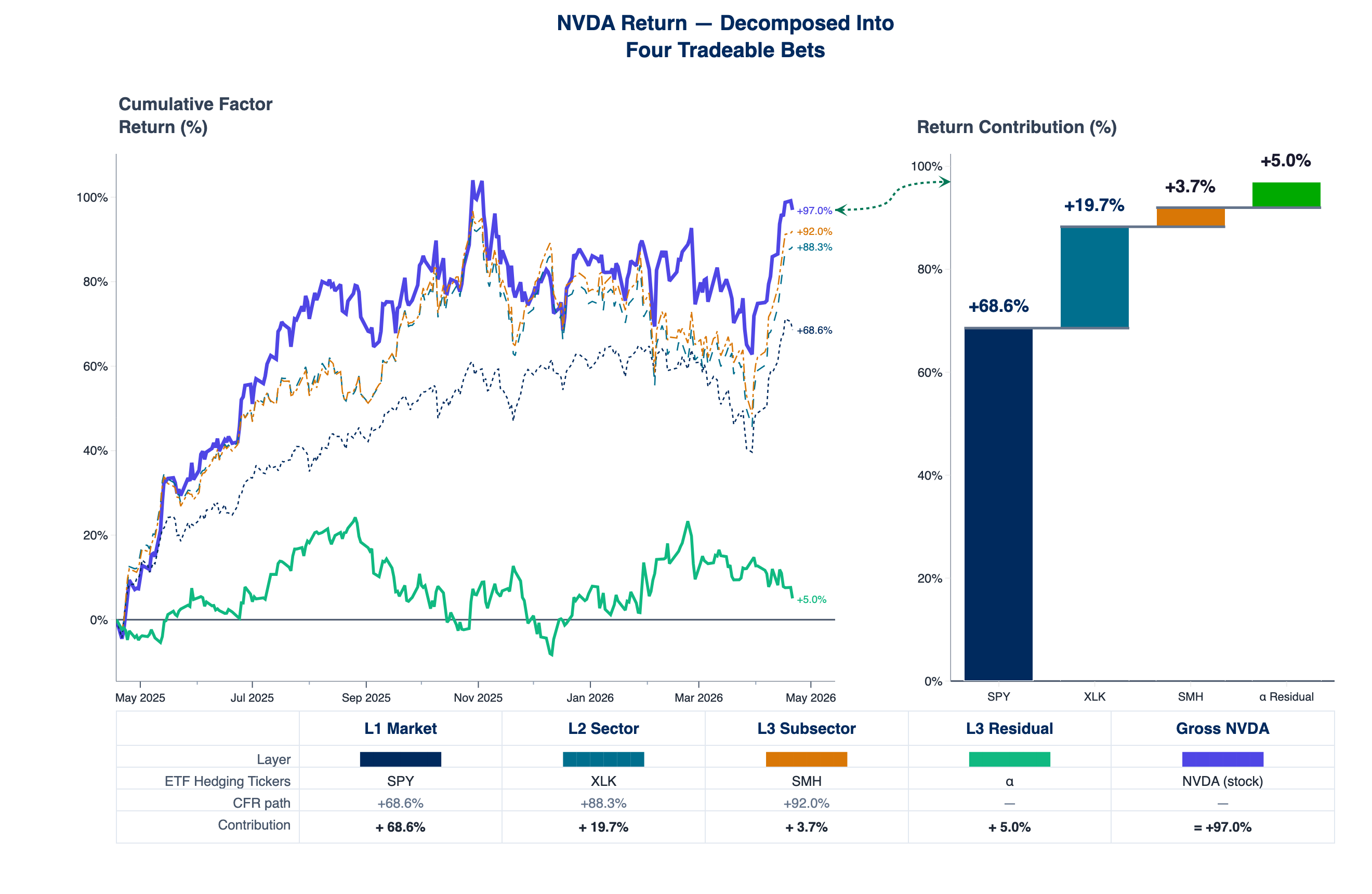
Each number in the decomposition corresponds to a priced, executable decision. A PM targeting semiconductor exposure without broad-market beta reads the required SPY short notional directly off the L1 layer. A PM evaluated on idiosyncratic return reads the residual as the portion of the year's return attributable to owning this specific name rather than its factor basket. The same decomposition drives both return and risk, so sizing and hedging come from the same object.
The subsector layer should be read as the dominant tradable proxy between sector and stock-specific residual, not as a claim of perfect classification. Mappings are imperfect, ETF baskets overlap, and some of what belongs to the subsector will show up in residual. The point is not to eliminate that leakage but to make the four layers — and the instruments that replicate them — explicit enough to size and hedge.
Two PMs ask the same question — "give me more tech" — and buy different stocks. The cascade shows they did not buy the same thing.
Same "tech" label, different bets: AAPL vs NVDA
Two PMs at the same firm want more tech. One adds AAPL, one adds NVDA. Sector screens read both as Technology, overweight, and a portfolio-down model registers both as the same technology loading. Sized at equal $-risk contribution — so NVDA's ~35% vol vs AAPL's ~23% is off the table — the per-dollar sector exposure differs by roughly an order of magnitude (near-zero vs ~22% explained risk on L2).
| (per unit of $-risk added, explained risk by layer) | AAPL | NVDA |
|---|---|---|
| Market (SPY) | 46.0% | 49.4% |
| Sector (XLK, net of market) | 0.4% | 21.5% |
| Subsector (net of sector) | 0.7% | 0.0% |
| Residual (idiosyncratic) | 52.9% | 29.0% |
Explained risk by layer, 2025-04-21 → 2026-04-21.
The shape of what each PM actually bought is almost entirely different:
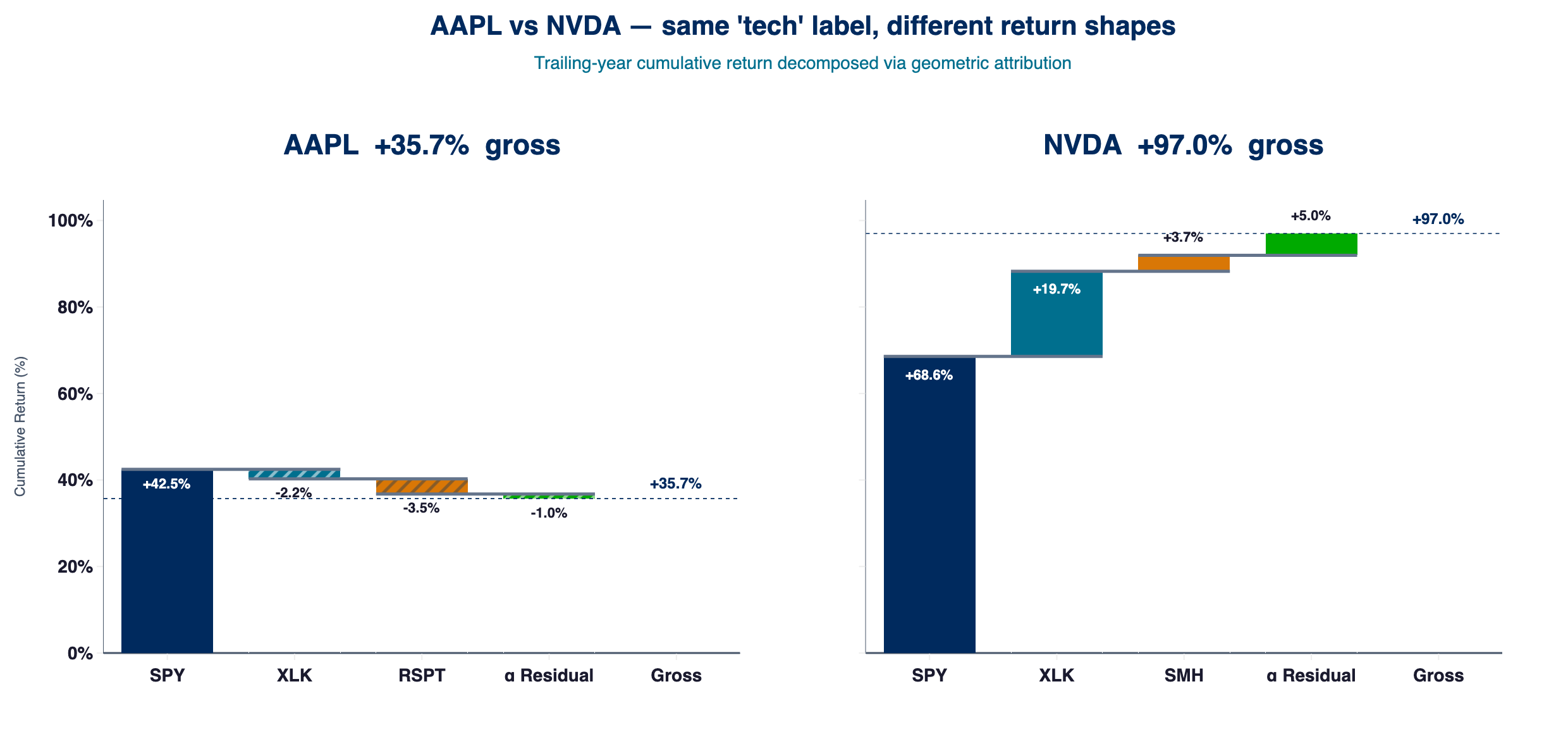
2025-04-21 → 2026-04-21, shared y-axis. AAPL: gross +35.7pp, SPY +42.5pp, XLK −2.2pp, RSPT −3.5pp, residual −1.0pp. NVDA: gross +97.0pp, SPY +68.6pp, XLK +19.7pp, SMH +3.7pp, residual +5.0pp. Layer attribution under the current ERM3 vintage; the Medium edition shows the April 2026 fit.
AAPL's L1 path alone (+42.5pp) exceeded its gross return; the tech and sub-tech layers were marginally negative and the residual near zero. NVDA's factor layers show large return contributions in the waterfall; explained risk at L3 is still a thin slice (correlation stacks most variance in market, sector, and residual in this window). The residual added a further +5.0pp on top of that factor stack.
If the thesis is "I want more tech", AAPL is not a clean instrument for that thesis. The clean sector-only instrument is XLK stripped of market beta — exactly what the cascade's L2 layer isolates. If the thesis is "I want more semiconductors", the instrument is NVDA or SMH, with SPY and XLK hedges specified directly from the cascade. Same label. Different bet.
This is consistent with evidence that much of the active risk in concentrated books is idiosyncratic rather than factor-driven (Cremers & Petajisto 2009; Kacperczyk, Sialm & Zheng 2005).
Same "energy" label, opposite bets: XOM vs KMI
Two PMs want more energy exposure. One adds XOM (largest integrated major in the S&P 500). One adds KMI (Kinder Morgan, one of the largest midstream pipelines, also S&P 500). On a sector screen, both read Energy, overweight. The cascade shows they are almost opposite bets (2025-04-21 → 2026-04-21, risk attribution):
| XOM | KMI | |
|---|---|---|
| Market (SPY) | 3.7% | 10.4% |
| Sector (XLE, net of market) | 78.3% | 16.9% |
| Subsector (net of sector) | 0.3% | 10.6% |
| Residual (idiosyncratic) | 17.7% | 62.0% |
| Ann. daily vol | 34.2% | 19.0% |
XOM puts about three-quarters of its risk in the sector layer — in the table, 78.3% explained risk on L2 (XLE net of SPY) — so in risk terms it behaves like an XLE proxy. A PM targeting pure oil-sector beta gets that exposure directly; one targeting something more specific does not.
KMI is the inverse: 16.9% sector, 10.6% midstream-specific (AMLP), and 62.0% idiosyncratic — Kinder-Morgan-specific drivers (fee structure, project mix, regulatory) that no ETF captures. A PM who added KMI for oil exposure is mostly holding a pipeline business with large company-specific risk.
The same cascade applied to returns makes the divergence concrete:
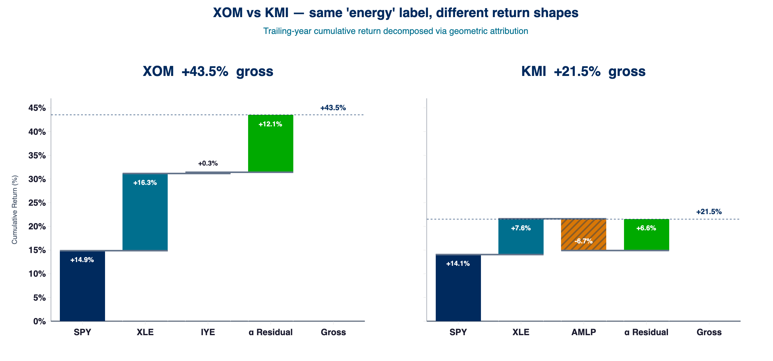
2025-04-21 → 2026-04-21, shared y-axis. XOM: gross +43.5pp, SPY +14.9pp, XLE +16.3pp, IYE (broad-energy, overlaps XLE) +0.3pp, residual +12.1pp. KMI: gross +21.5pp, SPY +14.1pp, XLE +7.6pp, AMLP (midstream subsector) −6.7pp, residual +6.6pp. Layer attribution under the current ERM3 vintage; the Medium edition shows the April 2026 fit.
XOM's cascade is concentrated in two layers: XLE +16.3pp and residual +12.1pp, together roughly twice the combined contribution of the other two. Predominantly sector, with a meaningful XOM-specific component. KMI's profile is the inverse: a low-double-digit SPY contribution, +7.6pp from XLE, a −6.7pp midstream drag (AMLP), and a +6.6pp residual that offsets the midstream drag and returns the position to a positive gross.
The same lens across the Magnificent Seven
Running the same decomposition across MAG7 produces seven distinct exposure profiles under a single Technology label (2025-04-21 → 2026-04-21), sorted below by idiosyncratic share — the component a stock-picking mandate is compensated for:
| Name | Dominant Subsector ETF | What You're Actually Holding |
|---|---|---|
| AAPL | RSPT | Most idiosyncratic of the seven — nearly three-quarters of risk is name-specific, not the shared cascade. |
| GOOG | FDN | About two-thirds name-specific — second only to AAPL. |
| META | FDN | Same sleeve as GOOG, slightly lower idio — more co-movement with the shared sleeve. |
| MSFT | IGV | Same idio share as META, different composition — more of the risk budget loads on the application stack than on hardware breadth. |
| AMZN | XRT | Mid-pack; diversified operating mix shows up as more factor, less residual than the top three. |
| TSLA | CARZ | Nearly half idiosyncratic — cycle and cap-structure risk still sit heavily in the systematic layers. |
| NVDA | SMH | Least idiosyncratic here — the name trades like the dominant industry factor; residual is the smallest slice of the seven. |
Idiosyncratic share spans 45% to 73% across the seven names, and the dominant subsector differs for each. A PM targeting semiconductor exposure has a direct instrument pairing (NVDA, or SMH as the ETF proxy). A PM targeting systems-software exposure does not get it from AAPL, AMZN, or NVDA — only from MSFT or IGV. The cascade makes the mapping from thesis to instrument explicit for each position.
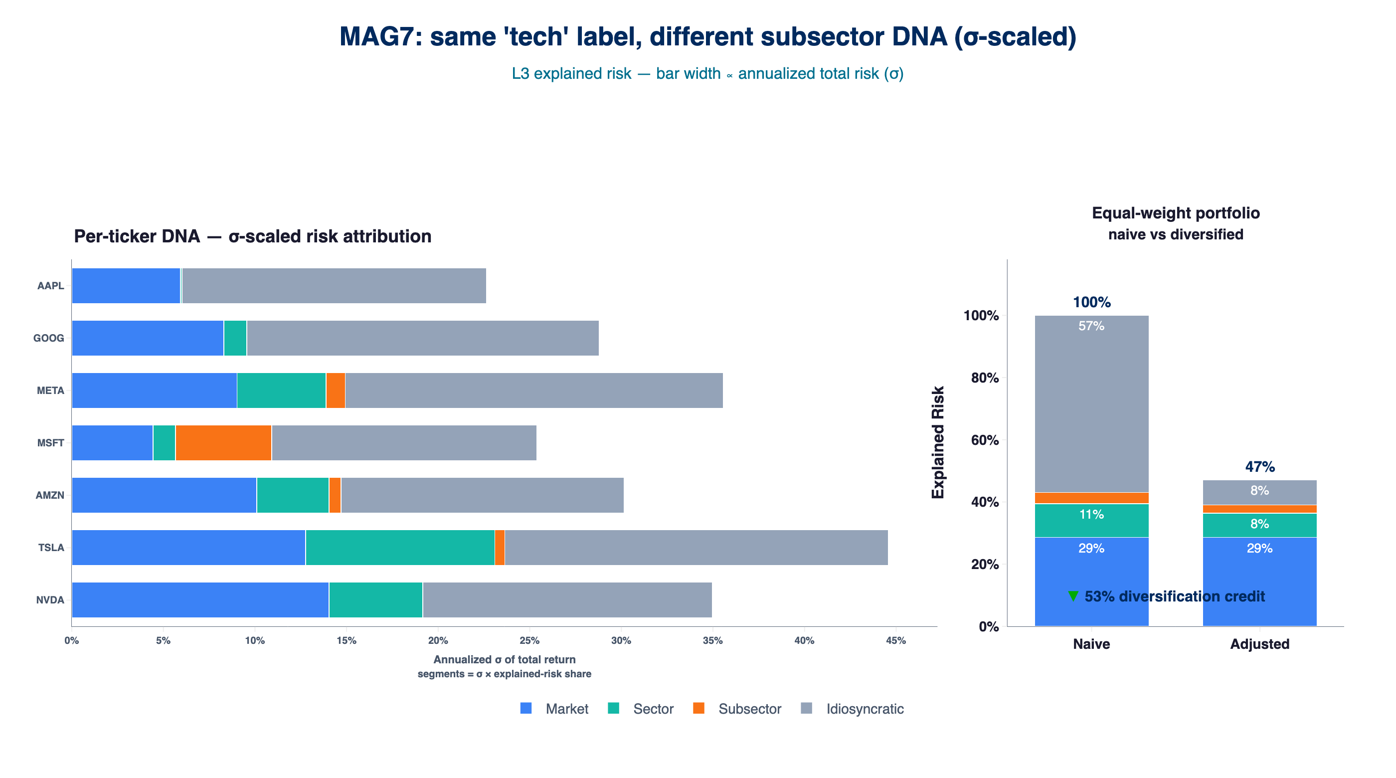
Left Side: per-ticker σ-scaled risk attribution — each segment width = σ × explained-risk share, so names with the same DNA mix but different total risk no longer look identical.
Right Side: equal-weight MAG7 portfolio, naive (position-weighted sum, 100%) versus correlation-adjusted (47%). Layer attribution under the current ERM3 vintage; the Medium edition shows the April 2026 fit.
The Idiosyncratic layer collapses from 57% to 8% as cross-stock correlation diversifies stock-specific risk away; the Market layer stays at 29% because systematic risk is not diversifiable within a long-only sector-concentrated book.
The right panel reframes the usual diversification intuition. An equal-weight MAG7 book collapses the idiosyncratic component — the layer where stock-picking edge accumulates — from 57% of naive weighted risk to 8% of adjusted portfolio risk. For a PM evaluated on residual return, equal-weighting across MAG7 diversifies away the layer the mandate is paid for. The market component (~29%) is unaffected: systematic risk is not diversifiable within a long-only sector-concentrated book, so SPY overlay remains the only instrument that moves it.
Portfolio-down and position-up as complements
All the established factor-model vendors — Barra, Axioma, Bloomberg MAC3 — start from a shared library of factors to build a covariance structure, which ultimately produces derived position-level statistics. That framing is native to the aggregate question: how is the book tilting, what is its tracking error, and where did returns come from in factor terms.
Position-up starts at the other end — computing explained variance through a series of orthogonal regressions that produce additive risk and return components. From this approach, the portfolio view falls out as a consequence of those layers, rather than as a substitute for them.
The two approaches answer different questions. Portfolio-down explains the book. Position-up explains what you actually bought. A risk program that reads both is strictly better informed than one that reads only one.
Position-up decomposition doesn't rely on a pre-specified, vendor-maintained, and ever-expanding library of style factors. Much of what gets labeled as the "factor zoo" is already sitting in plain sight — embedded in sector and subsector exposures as tradable risk. The proliferation of factors is often a labeling exercise layered on top of effects that are already there. This framework doesn't assume the zoo — it lets those effects show up where they actually live.
Position-up also removes the need to force every thesis into an expanding factor taxonomy. The residual is not a modeling gap to be minimized — it is the portion of risk and return that cannot be rented from a factor and must come from the position itself. That is the bet.
Macro & style: gross vs L3 residual (reporting bridge)
The cascade above assigns market, sector, and subsector to listed ETFs with explained risk and hedge ratios. Style and macro labels do not, in general, get a parallel tradeable sleeve at the intersection of factor and subsector — there is no single ETF that encodes "value × this subsector" or most macro crosses. This exhibit is intentionally lighter: correlations of each factor with gross returns versus with the L3 residual only (the name after the three tradeable layers are stripped). There is no added regression rung for these factors, no extra explained-risk slot, and no hedge ratio — the point is insight and reporting, not an additional hedge leg.
Read it as a bridge to how portfolio-down analytics and committees already discuss Fama–French–style tilts and macro exposures, mapped onto the same L3 residual you treat as the stock-specific bet. Each arrow runs from gross correlation (open circle) to L3 residual correlation (filled circle); the chart highlights the two MAG7 names with the largest absolute shift between those two readings per factor.
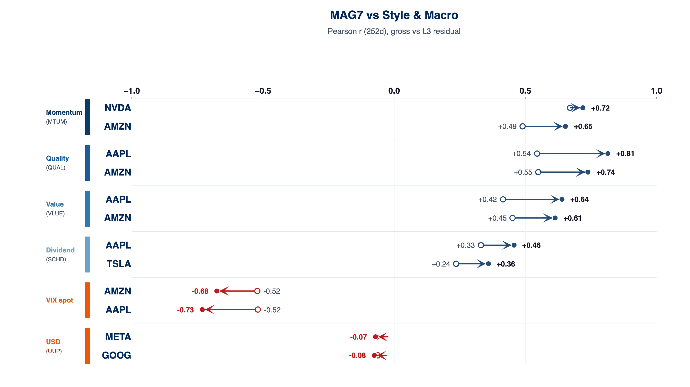
2025-04-21 → 2026-04-21, Pearson correlation over trailing 252 days.
Residualization can strengthen a factor correlation just as easily as it weakens one — a loading portfolio-down analysis can understate or overstate because SPY absorbs part of the correlation before the factor model sees it.
Implications for sizing, hedging, and conviction
Once each position is decomposed into additive, orthogonal layers, three decisions become explicit: what exposure you are buying, how you hedge it, and how much residual risk you are willing to own.
Sizing becomes an exposure decision rather than a dollar allocation, because the per-dollar composition of each layer is known.
Hedging is specified at the level of the exposure itself — SPY against L1, a sector ETF against L2 — rather than applied generically at the book level.
Conviction is the size of the residual bet.
Without this decomposition, the link between thesis, instrument, and hedge remains implicit. RiskModels.app makes it explicit — returning position-level exposures, hedge ratios, and residual contributions in real time, so sizing and hedging decisions can be specified directly rather than inferred. The result is not a different view of risk — it's one you can actually trade.
Access is API-first — designed to be called directly inside research and PM workflows — so the decomposition becomes part of how positions are evaluated, not a report that gets read after the fact.
Methodology — regression windows, subsector proxy selection, and orthogonalization mechanics — is covered in later parts of this series and at riskmodels.app/docs.
Next in the series: Linking Portfolio Risk Metrics to Investment Process — talking to your book the way you already talk to your analysts.
Further reading
Orthogonal decomposition and additive variance
- Frisch, R. & Waugh, F.V. (1933). "Partial Time Regressions as Compared with Individual Trends." Econometrica 1(4): 387–401. Lovell, M.C. (1963). "Seasonal Adjustment of Economic Time Series and Multiple Regression Analysis." JASA 58(304): 993–1010. The Frisch–Waugh–Lovell theorem: regression coefficients from sequential net-of-prior-regressor residualization equal those from full joint regression — the mathematical basis for additive, layer-wise variance decomposition.
- Klein, R.F. & Chow, V.T. (2013). "Orthogonalized factors and systematic risk decomposition." Quarterly Review of Economics and Finance 53(2): 175–187. Direct precedent for decomposing systematic risk via orthogonalized factors.
Factor model foundations
- Rosenberg, B. (1974). "Extra-Market Components of Covariance in Security Returns." Journal of Financial and Quantitative Analysis 9(2): 263–274. The Barra-lineage paper; the canonical portfolio-down framing.
- Connor, G. (1995). "The Three Types of Factor Models: A Comparison of Their Explanatory Power." Financial Analysts Journal 51(3): 42–46.
- Grinold, R.C. & Kahn, R.N. (2000). Active Portfolio Management (2nd ed.). McGraw-Hill. The practitioner source for residual return as the object of active skill.
The factor zoo
- Harvey, C.R., Liu, Y. & Zhu, H. (2016). "…and the Cross-Section of Expected Returns." Review of Financial Studies 29(1): 5–68.
- Feng, G., Giglio, S. & Xiu, D. (2020). "Taming the Factor Zoo: A Test of New Factors." Journal of Finance 75(3): 1327–1370.
- McLean, R.D. & Pontiff, J. (2016). "Does Academic Research Destroy Stock Return Predictability?" Journal of Finance 71(1): 5–32.
Concentrated books and idiosyncratic risk
- Cremers, K.J.M. & Petajisto, A. (2009). "How Active Is Your Fund Manager? A New Measure That Predicts Performance." Review of Financial Studies 22(9): 3329–3365.
- Kacperczyk, M., Sialm, C. & Zheng, L. (2005). "On the Industry Concentration of Actively Managed Equity Mutual Funds." Journal of Finance 60(4): 1983–2011.
- Van Nieuwerburgh, S. & Veldkamp, L. (2010). "Information Acquisition and Under-Diversification." Review of Economic Studies 77(2): 779–805.